In the following detailed example, we show a typical application of GRTOOL using the standard EMME/2 demonstration data bank with the Winnipeg network.
First, the emissions for carbon monoxide, hydrocarbons and nitrous oxides
are computed using the network calculator, module 2.41, and
the resulting emissions are saved in the link extra attributes @co,
@hc and @nox. For the sake of
this example, functions were used which are based on the values published
by the Swiss Federal Office for the Protection of the Environment for private
vehicles for the year 1984.
![]() .
These functions are fourth degree polynomials of the travel speed in km/h
on the link which yield the amount of pollutants generated by one vehicle
in g/km.
.
These functions are fourth degree polynomials of the travel speed in km/h
on the link which yield the amount of pollutants generated by one vehicle
in g/km.
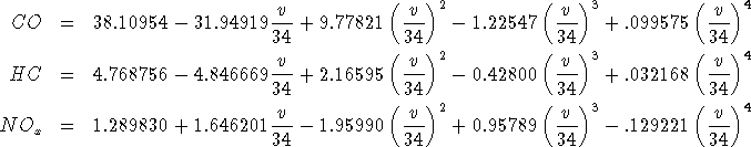
Since distances in the Winnipeg data bank are given miles, care must be taken regarding the units when applying the above formulae.
Once the emissions are computed at the link level and saved in the corresponding extra attributes, macro GRMACRO is called from the main menu as follows
~<grmacro .01 @co @hc @nox
When GRMACRO is running, the user is prompted to specify, in the usual manner, the subset of links to include in the link data file. Also, since the macro is started from the main menu, the user is asked to specify the name of the output file to be generated. The following shows the screen output generated in this example by GRMACRO:
Enter: Next module=~<grmacro .01 @co @hc @nox
*********************** GRMACRO (2.1) *****************************
GRMACRO - macro to generate link data file for use with GRLINK

Usage: ~<grmacro <width> <val1> <val2> <val3> ...

where   <width>  constant or link attribute containing link width
        <valK>   link attribute containing link data K

Notes: - macro is started from main menu or primary select of 2.41
       - tmpl9 is used to store link widths
       - link subset and name of output file is asked interactively
       - switch 22 should be off in order to avoid eng. notation
*******************************************************************

result    =   0 * (xi + yi + xj + yj + tmpl9) + @co + @hc + @nox

Enter: Selected link types or attributes (from, to)
= >>ci=0
= >>and cj=0
= >>
Enter: Name of link data file to be generated= >>emission.lnk

Macro ``~<grmacro .01 @co @hc @nox'' terminated normally.
*******************************************************************
Enter: Next module=
The generated link data file is called emission.lnk and contains
the coordinates, widths and specified link attributes for the selected links,
as shown below:
inode jnode     xi     yi     xj     yj tmpl9     @co     @hc    @nox    result
  165   166   .773   .848   .903   .961   .01  .69519  .09486   .1961    .98615
  165  1055   .773   .848    .61   .669   .01 11.6673 1.33537 1.46016   14.4629
  166   165   .903   .961   .773   .848   .01 5.07276   .5806  .63485   6.28821
  166   167   .903   .961   .951  1.042   .01  .62567  .08537  .17649    .88754
  167   166   .951  1.042   .903   .961   .01 4.56548  .52254  .57137   5.65939
  167   168   .951  1.042      1  1.107   .01  .41711  .05692  .11766    .59169
 ......
 1064  1063   .578  -.305   .432  -.289   .01 12.3012 1.42774   .8722   14.6011
 1065   477 -3.643  -9.56 -1.744 -9.349   .01  .29588  .04677  .12603    .46867
 1065   546 -3.643  -9.56  -8.79 -9.089   .01   .8352  .13201  .35575   1.32297
 1066   727 -2.059   .674 -2.038   .969   .01 3.84376  .44217  .51005   4.79599
 1067   493  -2.02 -4.056 -2.004 -4.299   .01 4.90105  .60934 1.00488   6.51527
 1067   494  -2.02 -4.056 -2.004 -3.634   .01 1.55136   .2348  .58801   2.37417
This link file emission.lnk is now converted to a grid with
a cell size of 0.5 x 0.5 miles. This is achieved by calling the program
GRLINK as follows:
grlink emission.lnk 0.5 emission.grd
The resulting grid data file emission.grd contains the grid cell
values of same variables as contained in the link file.
# Created by GRLINK (2.1)
  xg=0.5   yg=0.5      @co      @hc     @nox   result
   0.000    0.000   41.108    4.755    3.980   49.843
   0.000    0.500   69.116    7.955    8.200   85.271
   0.000    1.000   19.950    2.367    3.142   25.459
   0.000    1.500   28.703    3.358    4.063   36.124
   0.000    2.000    6.053    0.690    0.702    7.444
   0.000    2.500   13.790    1.584    1.523   16.897
   0.000    3.000    7.207    0.833    0.570    8.610
   0.000    3.500    0.506    0.058    0.066    0.630
   0.000    4.000    1.593    0.183    0.212    1.989
   0.000    4.500    0.023    0.004    0.009    0.036
   0.000    5.000    6.533    0.837    1.503    8.873
   0.000    5.500    0.179    0.023    0.041    0.242
   0.000    7.000    0.514    0.081    0.219    0.814
   0.000   -0.500   81.059    9.301    7.771   98.130
   0.000   -1.000  107.999   12.425    9.706  130.130
   0.000   -1.500   49.093    5.690    4.383   59.166
   0.000   -2.000    8.431    0.977    0.667   10.074
   0.000   -2.500   23.692    2.731    1.988   28.411
......
The emission values contained in the file emission.grd can now be
displayed in the form of annotations which are generated with program
GRANNOT. But in order to run GRANNOT, it is first necessary to prepare
the corresponding graphic parameter files. This is best done using
the program GRPARAM.
The first example of the generation of such a parameter file is for generating a display of the type shown before,
dividing the grid cells into 5 different classes according to the emission levels:
Enter: Name of existing parameter-file for default values (optional)=
Enter: Name of parameter-file to be generated = co.par
Enter: Horizontal[,vertical] grid distances (1,1) = .5 .5
Draw complete grid (n) ? n
Enter: Grid color (4) = 4
Enter: Name or number of data item to be displayed (1) = @co
Select: Type of gird representation
        1= Classes defined by value interval
        2= Numeric values
        3= Hatching with proportional density
       (1) 1
Select: Type of legend
        1= None
        2= Default
        3= Customized
       (1) 2
Enter: Text for legend title (*) = CO:
Enter: Lower left corner of first legend box (xl, yl) (*,*) = 6.5,5
Enter: Number of classes (0) = 5

Enter: Class interval  1: (from, to) (0, 0) =0 5
Enter: Color for class  1 (0) = 5
Select: Hatching pattern for class  1
        1= Horizontal lines
        2= Vertical lines
        3= Horizontal and vertical lines
       () 3
Enter: Distance between 2 horizontal lines (0) = .25
Enter: Distance between 2 vertical lines (0) = .25
Enter: Text for class  1 () =   < 5 KG

Enter: Class interval  2: (from, to) (0, 0) =5 10
Enter: Color for class  2 (0) = 3
Select: Hatching pattern for class  2
        1= Horizontal lines
        2= Vertical lines
        3= Horizontal and vertical lines
       () 3
Enter: Distance between 2 horizontal lines (0) = .125
Enter: Distance between 2 vertical lines (0) = .125
Enter: Text for class  2 () =  5-10 KG

Enter: Class interval  3: (from, to) (0, 0) =10 20
Enter: Color for class  3 (0) = 7
Select: Hatching pattern for class  3
        1= Horizontal lines
        2= Vertical lines
        3= Horizontal and vertical lines
       () 3
Enter: Distance between 2 horizontal lines (0) = .0625
Enter: Distance between 2 vertical lines (0) = .0625
Enter: Text for class  3 () = 10-20 KG

Enter: Class interval  4: (from, to) (0, 0) =20 40
Enter: Color for class  4 (0) = 8
Select: Hatching pattern for class  4
        1= Horizontal lines
        2= Vertical lines
        3= Horizontal and vertical lines
       () 3
Enter: Distance between 2 horizontal lines (0) = .03125
Enter: Distance between 2 vertical lines (0) = .03125
Enter: Text for class  4 () = 20-40 KG

Enter: Class interval  5: (from, to) (0, 0) =40,999999
Enter: Color for class  5 (0) = 2
Select: Hatching pattern for class  5
        1= Horizontal lines
        2= Vertical lines
        3= Horizontal and vertical lines
       () 3
Enter: Distance between 2 horizontal lines (0) = .015625
Enter: Distance between 2 vertical lines (0) = .015625
Enter: Text for class  5 () =   >40 KG
The result of the above executing of GRPARAM is a graphic parameter file
co.par with the following contents:
GD         .5         .5 Horizontal,vertical grid distances
CG          0            Draw complete grid
GC          4            Grid color
DN        @co            Name or number of data item to be displayed
RP          0            Representation (0=Class,1=Numbers,2=Proportional)
LG          1            Legend (0=None,1=Default,2=Customized)
LT 'CO:'                 Legend title
LK        6.5          5 Lower left corner of first legend box (xl, yl)
NC          5            Number of classes
LC  1         0         5   5    .25    .25 '  < 5 KG'
LC  2         5        10   3   .125   .125 ' 5-10 KG'
LC  3        10        20   7  .0625  .0625 '10-20 KG'
LC  4        20        40   8  .03125  .03125 '20-40 KG'
LC  5        40    999999   6  .015625  .015625 '  >40 KG'
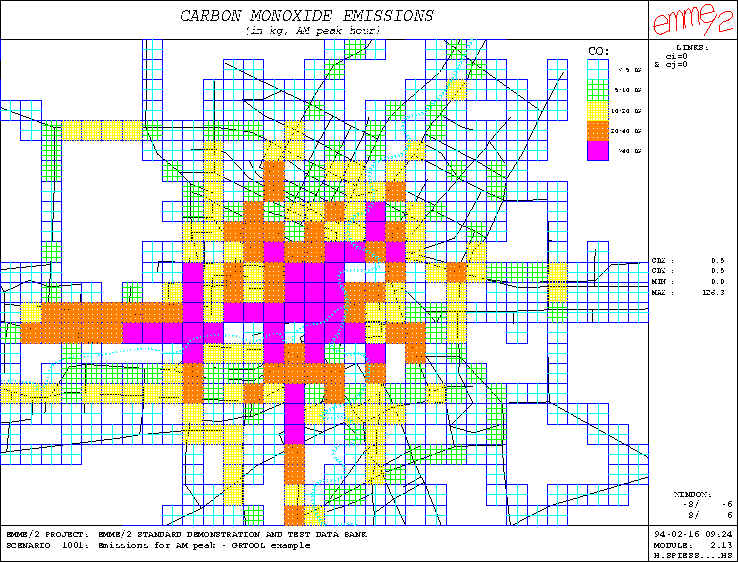
Figure 1: Example of grid representation by interval classes
Using the resulting graphic parameter file co.par the program GRANNOT
is now used to produce an annotation file annotc using the command
grannot co.par emission.grd annotc
which can be superimposed on an EMME/2 network plot to obtain the map of carbon monoxide emission levels shown in in Figure 1.
The second example output is a grid display of the hydrocarbon emission in which the amount of generated pollutants is displayed numerically in each grid cell. For the purpose, a new graphic parameter file is created with GRPARAM in the following way:
Enter: Name of existing parameter-file for default values (optional) =
Enter: Name of parameter-file to be generated = hc.par
Enter: Horizontal[,vertical] grid distances (1,1) = .5 .5
Draw complete grid (n) ? n
Enter: Grid color (4) =
Enter: Name or number of data item to be displayed (1) = @hc
Select: Type of gird representation
        1= Classes defined by value interval
        2= Numeric values
        3= Hatching with proportional density
       (1) 2

Enter: Color of the numbers (4) = 2
Enter: Text size of the numbers (*) = -.12
Enter: Minimal field width (*) = 3
Enter: Number of digits after decimal point (*) = 1
Enter: Offset of the number inside grid box (xdisp, ydisp) (*,*) = .26 .17
Note that the negative character size implies horizontal centering at the specified offset.
The resulting graphic parameter file hc.par contains the following
information:
GD         .5         .5 Horizontal,vertical grid distance
CG          0            Draw complete grid
GC          4            Grid color
DN        @hc            Name or number of data item to be displayed
RP          1            Representation (0=Class,1=Numbers,2=Proportional)
PC          2            Color of the numbers
NS       -.12            Text size of the numbers
DT          3            Minimal field width
DF          1            Number of digits after decimal point
DG        .26        .17 Offset of the number inside grid box (xdisp, ydisp)
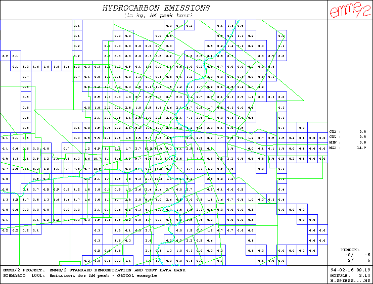
Figure 2: Example of grid representation using numerical values
Running the command
grannot hc.par emission.grd annoth
produces the annotation annoth. This annotation is shown in Figure
2; it is displayed here without the
underlying network, but with the zone boundaries instead.
Finally, to finish this series of output examples, a graphic parameter file is created to represent the nitrous oxides levels using proportional hatching. In this type of representation, the number of hatch lines in each grid cell is proportional to the corresponding data value. A scale factor 1 is used here, implying that each vertical line corresponds to 1 kg of pollutant. The following shows the dialog generated by GRPARAM:
Enter: Name of existing parameter-file for default values (optional) =
Enter: Name of parameter-file to be generated = nox.par
Enter: Horizontal,vertical grid distance (1,1) = .5 .5
Draw complete grid (n) ? n
Enter: Grid color (4) = 4
Enter: Name or number of data item to be displayed (1) = @nox
Select: Type of gird representation
        1= Classes defined by value interval
        2= Numeric values
        3= Hatching with proportional density
       (1) 3

Enter: Scale factor () = 1
Enter: Color of pattern (4) = 3
The resulting parameter file nox.par contains the following records:
GD         .5         .5 Horizontal,vertical grid distance
CG          0            Draw complete grid
GC          4            Grid color
DN       @nox            Name or number of data item to be displayed
RP          2            Representation (0=Class,1=Numbers,2=Proportional)
SC          1            Scale factor
PC          3            Color of pattern
Running the command
grannot nox.par emission.grd annotn
produces the annotation annoth. This annotation is shown in Figure
3; it is displayed here on top of a bandwidth plot of the auto
volumes produced with EMME/2 module 6.12.
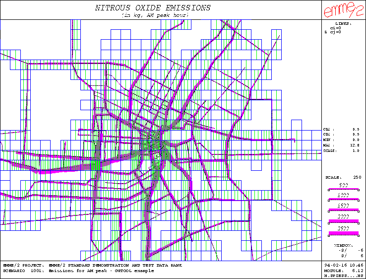
Figure 3: Example of grid representation using proportional hatching