On Algorithms for the Traffic Assignment Problem

Although the linear approximation algorithm for obtaining the solution of the equilibrium traffic assignment problem is known since 1974 and it has been implemented in several codes (EMME/2, as well as the UROAD module of UTPS, among others), there are still other algorithms used to obtain solution to this problem. Some of the more popular are incremental assignment, capacity restraint and the successive average method. The purpose of this note is to show that the results obtained with the latter methods only approximate the solution of the equilibrium traffic assignment problem.

The behavioral assumption of the equilibrium traffic assignment problem is that each user chooses the route that he perceives the best; if there is a shorter route than the one that he is using, he will choose it. This results in flows that satisfy Wardrop's "user optimal" principle, that no user can improve his travel time by changing routes. The consequence is that the equilibrium traffic assignment corresponds to a set of flows such that all paths used between an origin/destination pair are of equal time. We examine next the results produced for a simple example by the linear approximation method, incremental assignment, capacity restraint and the successive average method.

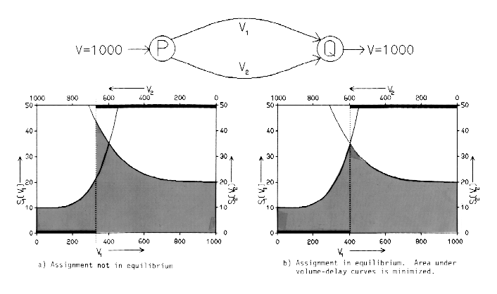
The solution to the equilibrium traffic assignment problem is equivalent to solving a problem where the area under the volume delay curves is minimized. This can be seen intuitively from the little example below.

The linear approximation method has the advantage that at each cycle (iteration), the total area under the volume-delay curves decreases and a measure of the difference between the current flows and the equilibrium flows can easily be estimated. It has the following general steps:

0 - Initialization

Initial solution is obtained by all-or-nothing assignment of demand g on shortest paths computed with arc costs :=s(0), i:=0.

1 - Update Link Costs

i:=i+1; :=s( ).

2 - Descent Direction

: all-or-nothing assignment of demand g on shortest path computed with arc costs .

3 - Compute Optimal Step Size

: for which the area under the volume-delay curves is minimized for the flow + ( - ), 0<= <=1.

4 - Update Link Flows

:= + ( - ).

5 - Stopping Criterion

If | - | > return to step 1 (total travel time still significantly different from total travel time on shortest paths), otherwise := , :=s( ) and STOP.

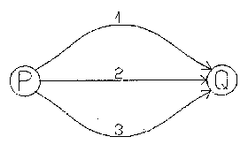
The example considered consists of three links with the travel time functions shown below. The demand is 1000 trips from P to Q.

The results obtained after the first nine iterations of the linear approximation method, as well as the optimal solution, where all paths used are of equal length are given in the table below.

0 10.00 20.00 25.00 1000 0 0 197500 1.00000

1 947.50 20.00 25.00 403 597 0 19740 0.59654

2 34.84 34.84 25.00 338 500 161 18999 0.16113

3 22.30 27.35 25.31 362 483 155 18945 0.03555

4 26.09 26.36 25.27 355 473 173 18936 0.02040

5 24.82 25.86 25.41 359 469 171 18934 0.00719

6 25.61 25.69 25.40 357 467 176 18933 0.00536

7 25.28 25.57 25.44 359 466 175 18933 0.00200

8 25.50 25.52 25.44 358 465 177 18933 0.00156

9 25.40 25.49 25.45 358 465 177 18933 0.00059

Opt.Sol. 25.46 25.46 25.46 358 465 177 18933 0.00000

The figures under the column indicated F(v) give the area under the volume-delay curves which is minimized where the flows are so-called "equilibrium" flows and all the paths used are of equal length.

The incremental method proceeds through the following general steps:

0 - Initialization

Define number of increments N, :=0; i:=0.

1 - Update Link Costs

i:=i+1; :=s( ).

2 - Load Increment of Demand

: all-or-nothing assignment of demand g/N on shortest path computed with arc costs .

3 - Update Link Flows

:= + .

4 - Stopping Criterion

If i<N return to step 1, otherwise := , :=s( ) and STOP.

The results obtained with the incremental assignment method where N is chosen to be 10 are given in the table below.

1 10.00 20.00 25.00 100 0 0 1002

2 10.09 20.00 25.00 200 0 0 2060

3 11.50 20.00 25.00 300 0 0 3456

4 17.59 20.00 25.00 400 0 0 5920

5 34.00 20.00 25.00 400 100 0 7920

6 34.00 20.01 25.00 400 200 0 9928

7 34.00 20.19 25.00 400 300 0 11977

8 34.00 20.95 25.00 400 400 0 14160

9 34.00 23.00 25.00 400 500 0 16652

10 34.00 27.32 25.00 400 500 100 19153

Solution 34.00 27.32 25.05 400 500 100 19153

It is easy to see that the flows resemble those obtained with the linear approximation method but the times are not equal on all the used links. Since the method is heuristic, there is no reason to anticipate that the flows will satisfy strictly the equilibrium conditions; the fact that the times may be quite different on the paths used makes it impossible to use the travel times for cost benefit analyses.

The capacity restraint method is probably one of the first heuristic methods used for the emulation of equilibrium flows. It proceeds through the following general steps:

0 - Initialization

Define number of iterations N. Initial solution is obtained by all-or-nothing assignment on shortest paths computed with arc costs :=s(0); i:=0.

1 - Update Link Costs

i:=i+1; :=0.75 +0.25 s( ).

2 - Load Demand

: all-or-nothing assignment on shortest path computed with arc costs .

3 - Stopping Criterion

If i<N return to step 1, otherwise := , :=s( ) and STOP.

As can be seen in the table of results below, this method produces flows which are quite different than the equilibrium flows.

0 10.00 20.00 25.00 1000 0 0 -

1 244.38 20.00 25.00 0 1000 0 -

2 185.79 49.30 25.00 0 0 1000 -

3 141.84 41.98 140.74 0 1000 0 -

4 108.88 65.79 111.81 0 1000 0 -

5 84.16 83.64 90.11 0 1000 0 -

6 65.62 97.03 73.83 1000 0 0 -

7 286.09 77.77 61.62 0 0 1000 -

8 217.07 63.33 168.21 0 1000 0 -

9 165.30 81.80 132.41 0 1000 0 -

10 126.48 95.65 105.56 0 1000 0 - Solutions

for N=9 13.66 27.32 26.81 250 500 250 19756

for N=10 10.00 57.08 26.81 0 750 250 26902

The last method which we will look at is the successive average method which is known to be a convergent method, but the convergence is very slow and there is no reasonable stopping criterion, other than an arbitrary number of iterations. The method resembles the linear approximation method, except that the step size, lambda, is arbitrarily fixed to yield a solution in which each of the all-or-nothing flows yi have the same weight. The general steps of the method are:

0 - Initialization

Define number of iterations N. Initial solution is obtained by all-or-nothing assignment of demand g on shortest paths computed with arc costs := s(0), i:=0.

1 - Update Link Costs

i:=i+1; := s( ).

2 - All-or-nothing Assignment

: load demand g on shortest path computed with arc costs .

3 - Compute Step Size

:= 1/(i+1).

4 - Update Link Flows

:= + ( - ).

5 - Stopping Criterion

If i<N return to step 1, otherwise := , :=s( ) and STOP.

Several iterations on this method yields the following results.

0 10.00 20.00 25.00 1000 0 0 197500

1 947.50 20.00 25.00 500 500 0 21592 0.50000

2 68.59 27.32 25.00 333 333 333 19582 0.33333

3 21.57 21.45 30.72 250 500 250 19756 0.25000

4 13.66 27.32 26.81 400 400 200 19190 0.20000

5 34.00 23.00 25.74 333 500 167 19016 0.16667

6 21.57 27.32 25.36 429 429 143 19484 0.14286

7 41.63 23.95 25.19 375 500 125 19001 0.12500

8 28.54 27.32 25.11 333 444 222 19006 0.11111

9 21.57 24.57 26.13 400 400 200 19190 0.10000

Solution 34.00 23.00 25.74 400 400 200 19190

It is easy to see that the method has a tendency to "oscillate" and after nine iterations the flows resemble the equilibrium flows but the times are quite different on the used links.

The conclusion to be drawn from this little exercise is that having many algorithms for the equilibrium traffic assignment is not a blessing. It suffices to have one that is robust and which has good theoretical foundation, good empirical convergence and a good stopping criterion.